In the last post I created a gif summarizing the HadCRUT4 sea-surface temperature (HadSST3) data as its data collection evolved over time.

The goal of the last post was simply to visualize presence of any temperature measurement in a given matrix gridcell for that year-month global snapshot. In this post I thought it’d be interesting to sum up the raw data per year-month snapshot to see how the raw data compare to the adjusted data for the global trends.

I’ve pasted in again the necessary code to get the HadSST3 data downloaded and ready for processing. As in last post, we’re starting off using the raw data provided by HadCRUT at their official page for HadSST, and then we’ll grab the adjusted data next for the comparison. Both the raw and adjusted data come as text files. But because the raw data comes is a year-month series of global 36-by-72 gridded matrices, we need to do some light parsing to get the text into a list of matrices.

Getting and Cleaning the HadSST3 raw data

pacman::p_load(tidyverse, curl)

home <- getwd()
temp <- tempfile()
url <- "http://hadobs.metoffice.com/hadsst3/data/HadSST.3.1.1.0/ascii/HadSST.3.1.1.0.unadjusted.zip"
curl_download(url,temp)
data <- readLines(unz(temp, "HadSST.3.1.1.0.unadjusted.txt"))
unlink(temp)
data[1:2]

# meta-data pattern defining when each new matrix begin
ii <- grepl("\\d+\\s+\\d{4}\\s+\\d+\\s+Rows", data)
counter <- 0
index <- rep(NA,length(ii))

for (j in 1:length(data)){
  if(ii[j]){
    counter=counter+1
    index[j]=counter
  } else {
    index[j] = counter
  } }

Parsing raw data and Aggregating the Global Trend

The main difference from the code I used last time for prepping the data for the gif is: now instead of looking the presence of the missing code -99.99 vs anything else in each year-month matrix and giving it a 0 if missing and 1 if not, we’re just going to changing -99.99 to NA so we can sum over the values in the matrix. The non-missing values are in Celsius anomalies from global average over the period 1961-1990.

dat_mat_measures <- lapply(split(data,index), function(x) {
    meta <- x[1]
    yr <- regmatches(meta,regexec("\\d{4}",meta))[[1]]
    mo <- regmatches(meta,regexec("\\d{1,2}",meta))[[1]][1]
    mo <- ifelse(as.integer(mo)<10,paste0("0",mo),mo)
    mx <- x[2:37]
    mx <- sapply(mx, function(y) {
      m <- as.numeric(strsplit(trimws(y),"\\s+")[[1]])
      ifelse(m==-99.99, NA,m) })
    
    m <- matrix(mx,36,72)
    colnames(m) <- c(paste0(seq(175,5,by=-5),"W"),0,paste0(seq(5,180, by=5),"E"))
    rownames(m) <- c(paste0(seq(85,5,by=-5),"S"),"Eq",paste0(seq(5,90, by=5),"N"))
  
    stats::setNames(list(paste0(yr,"/",mo),mean(m,na.rm = T),m)
                    , c("ym","mean", "raw") )
  }) %>% transpose()

At this step, I can’t tell you how handy I found purrr::transpose to be in inverting the list structures from year-month at level one in the list with values of interest at level 2, to having all the values of interest being level 1 lists with their year-months as values. Super convenient to then put these into a dataframe!!

ym_mean <- data_frame(ym = unlist(dat_mat_measures$ym),
                      mean = as.numeric( unlist(dat_mat_measures$mean) ) )

Getting/Joining HadSST3 adjusted global monthly data

The HadCRUT website has several resources I found helpful in explaining the main reasons for their needing to make adjustments to the raw data. I’d start with the FAQ page, but they’ve also release 2 white papers. To give you the basic gist: the first one deals with adjustments made to the data due to differences in methods of measuring the temperature of the water over time since 1880. The second paper deals with adjustments needed for some of the sampling problems the HadSST data.

I found all three resources quite helpful in explain why they’ve made adjustments to the raw data. The opening to the second white paper summarizes their case quite plainly:

“SSTs have been observed by diverse means in the past 160 years. As a result, measurements of SST recorded in historical archives are prone to systematic errors - often referred to as biases - that are of a similar magnitude to the expected climate change signal. That biases exist is well documented….”

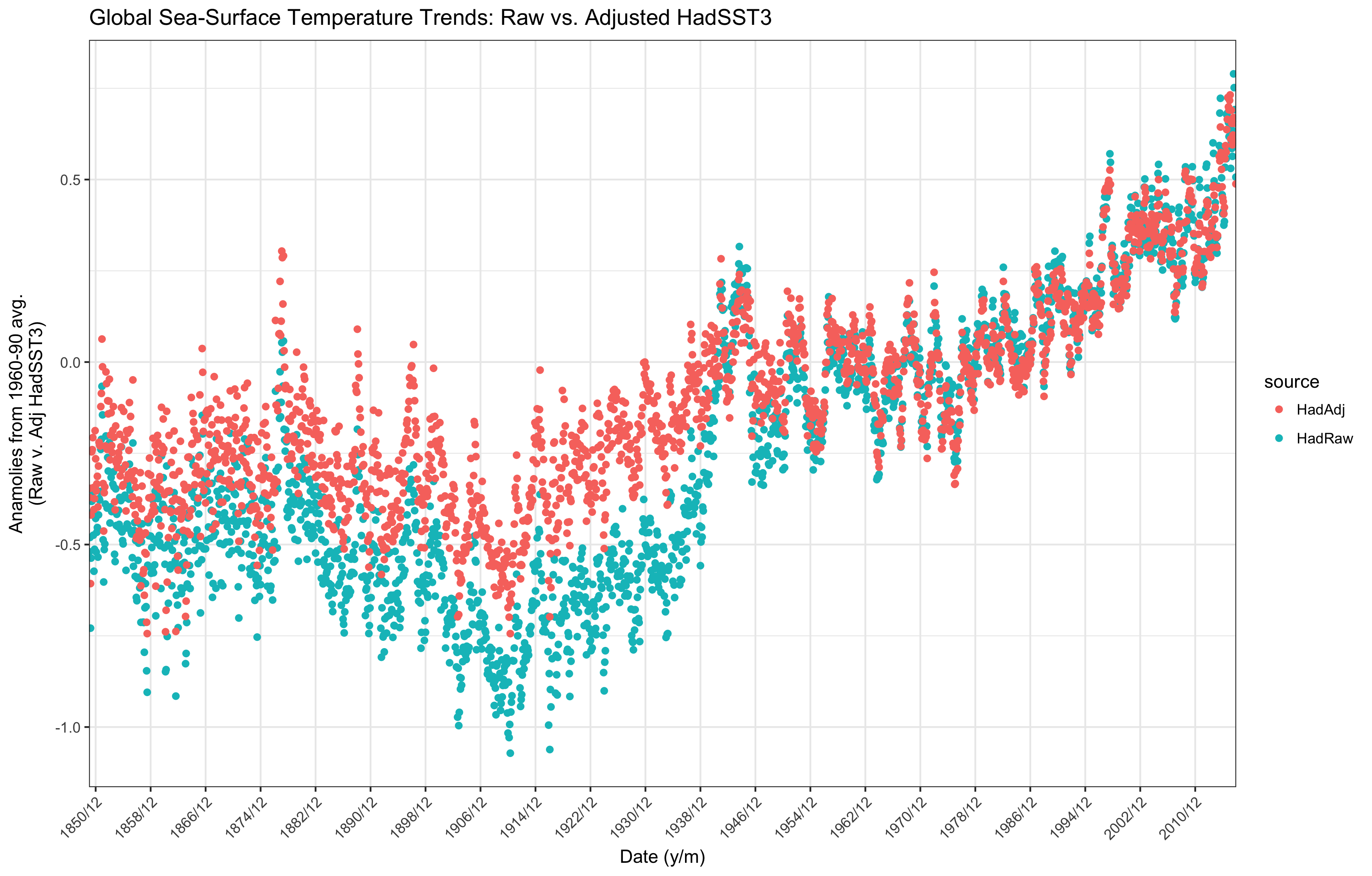
After reading that passage, I thought it would be useful to see how much “a similar magnitude to the expected climate change signal” actually looked like.

mon_gl <- "http://hadobs.metoffice.com/hadsst3/data/HadSST.3.1.1.0/diagnostics/HadSST.3.1.1.0_monthly_globe_ts.txt"
had_m_avg <- readLines(mon_gl)

had_m_avg2 <- lapply(had_m_avg, function(x) {#browser()
          v <-  strsplit(x,"\\s+")[[1]]
          data_frame(ym=v[1], avg=as.numeric(v[2]))
        }) %>% bind_rows()

raw_adj <- ym_mean %>%
  left_join(had_m_avg2, by="ym") %>%
  setNames(c("ym", "HadRaw", "HadAdj"))

ticks <- ym_mean$ym[seq(12,2000,by=96)]

raw_adj %>%
  mutate(ym=factor(ym,levels=ym, ordered=T)) %>%
  gather(source, temp, -ym) %>%
  mutate(source=factor(source)) %>%
  ggplot() + geom_point( aes(x=ym, y=temp,  color=source)) +
  ylab("Anamolies from 1961-90 avg.\n(Raw v. Adj HadSST3)") + xlab("Date (y/m)") +
  ggtitle("Global Sea-Surface Temperature Trends: Raw vs. Adjusted HadSST3") +
  scale_x_discrete(breaks = ticks) +
  theme_bw() + theme(axis.text.x = element_text(angle = 45, hjust = 1))

Some Comments

For ease of reading I reproduce the same plot again here.

As you can see, during the pre-1950ish part of the trend the raw data are uniformly cooler than the adjusted data. Post-1950ish the raw and adjusted data line up almost exactly. The gap in trends seems largest for the 1910-1950 period, witha max difference of around 0.48 Celsius (0.86 F).

raw_adj %>% summarize(max(HadAdj-HadRaw))

After reading the two white papers, as a matter of quick visual gut check for our own aggregation step it is encouraging to see in the plot agrees with the papers.

The FAQs do mention that the same adjustments are applied over the full trend, which was one of the HadSST3 improvements over the HadSST2 data. But it would appear that that the pre-1950ish data suffered from some data quality issues that the post-1950 data doesn’t: especially when temperature measuring methods allowed water to cool in the interim between when it was drawn from the water and when it was measured. Indeed, the first and second white papers detail several such sources and the ways in which they are addressed: interestingly, the reasons are a mix of technological and data provenance.

Spurred on by the closing statements of the second HadCRUT white paper,

“Until multiple, independent estimates of SST biases exist, a significant contribution to the total uncertainty will remain unexplored. This remains a key weakness of historical SST analysis.”

I’ll continue my exploration of the HadSST3 data and white papers. I encourage others who are using HadCRUT data, if you haven’t yet, to also read their suggested resources and dig into the raw data.