
Vocativ did an interesting analysis of the President’s State of the Union (SOTU) speeches, which we heard about via Partially Derative podcast. They showed that across the past couple hundred years and many Presidents, SOTU speeches have been targeted at audiences with lower and lower education levels.
Vocativ’s in-print interpretation of the downward sloping trend was that a speeches have gotten less sophisticated. Their recommended share-tweet for the article was more blunt:
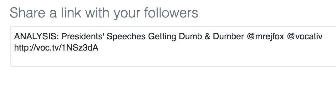
As does @partiallyd, we think there could be another interpretation: a growing populist bent in US culture that influenced even how POTUS did the SOTU. We try to test this hunch.
Idea
Tyler and I wanted to test for that broad cultural influence in other formal addresses. But what other kinds of speeches happen as regularly and consistently as SOTU? And then it struck us: commencement speeches! And what better test?
If commencement speeches are always targeted at an on-average relatively more educated audience of college graduates (and their families), then if we still see the same trend in language, this would be a fairly decent test that a cultural shift was influencing public address in general.
In the following series of posts, I’ll share the methods, data, and insights we found. We not only replicate Vocativ’s analysis, we extend it in several interesting ways, using different types of text analysis and a view inspired views of the data.
Methods
Commencing with Commencements.
Since the Vocativ article uses a common grade-level readability formula to measure the education level of the audience, all we really needed was to scrape some commencement addresses and apply the same readability algorithm. Also, we thought we’d extend the methodology by using several readability measures averaged together for robustness.
Data
Luckily for us, NPR had built a great web app to collect as many commencement addresses as they could readily find: 350+ speeches, in fact. So, with a bit of BeautifulSoup code (more on that to come!), we were able to scrape the website for many of the cool insights that data and portal afford.
First Results
But not to leave you hanging until our next post: when we compare our results (first graph above) to the interactive visualization that Vocativ produced, we do in fact find the same relative downward trend among the 280 usable speeches, from 12th grade level in the 1950s to 8th grade level in 2014. In this time series plot, we aggregate speeches by year, and scatter their occurrence with a trend line and bivariate correlation measure.
The negative time trend is not proof-positive of the populist interpretation, as opposed to a more curmudgeonly view on American education; but it is at least a stronger test than the original on new data and independent contexts. Finding the same results generalize across these instances, pretty much exactly, does say something for the populist interpretation.
The Code
We provide the code and data to reproduce the longitudinal readability graph below. The data provided is the output from the readability function in the GitHub readability package, not the raw text (we intend to release the full text based data set at the end of the blog series).
Load Packages & Data
if (!require('pacman')) install.packages("pacman")
pacman::p_load_gh("trinker/syllable", "trinker/readability")
pacman::p_load(dplyr, qdap, ggplot2, RCurl, readr, foreign)


## read in readability data
readability_scores_by_id_year <-
"https://raw.githubusercontent.com/trinker/data_store/master/readability_scores_by_id_year.csv" %>%
    getURL() %>%
    textConnection() %>%
    read.csv() %>%
    tbl_df()
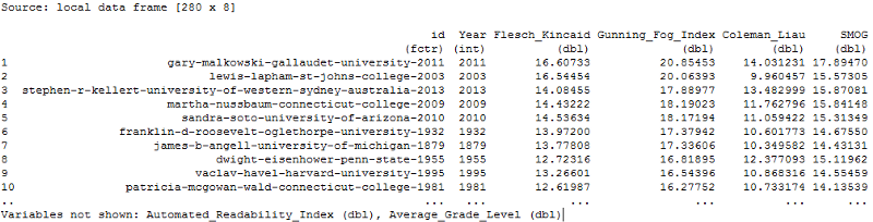
The output shows the speech id, year, 5 readability scores (Flesch Kincaid, Gunning Fog Index, Coleman Liau, SMOG, & Automated Readability Index), and an aggregate readability score. (Vocativ uses the first of the above five scores.) Readability scores are generally, computed from a combination of simple counts and ratios of a of characters, syllables, words, and sentences. The gist is that complex words and sentences make the comprehension of these texts more difficult.
Munging and Visualizing
To interpret the data we created the changes in speech readability over time visualization, using an aggregate of average grade level readability scores. Below, the dplyr & ggplot packages make light work of the data munging and plotting task.
readability_scores_by_id_year %>%
    group_by(Year) %>%
    summarize(
        Readability = mean(Average_Grade_Level),
        n = n()
    ) %>%
    ggplot() +
        geom_smooth(aes(x=Year, y=Readability), fill=NA, size=1,
            method='lm', color='blue') +
        geom_point(aes(x=Year, y=Readability, size=n), alpha=.3) +
        geom_point(aes(x=Year, y=Readability), size=1) +
        scale_size_continuous(range = c(3,10), name='N Speeches') +
        theme_bw() +
        theme(
            panel.grid.major.x=element_blank(),
            panel.grid.minor.x=element_blank(),
            panel.border = element_blank(),
            axis.line = element_line(color="grey50")
        ) +
        scale_x_continuous(
            expand = c(.01, 0),
            limits = c(1955, 2015),
            breaks = seq(1955, 2015, by=5)
        ) +
        ggtitle('Average Yearly Readability\nof Speeches Over Time') +
        annotate('text', x = 1962, y = 10.7,
            label = 'italic(r[xy] == -.299)',
            parse = TRUE, color='blue'
        )+
        ylab('Grade Level')
To Come in Future Posts
Next we hope to post about choices we made for scraping websites: specifically, how Python’s BeautifulSoup faired and what it was like to run the project on Jupyter/iPython Notebook vs an IDE.
In the meanwhile, go check out Tyler’s readability package and github star it for doing such a great job. Follow the button below.